What I want to find is:
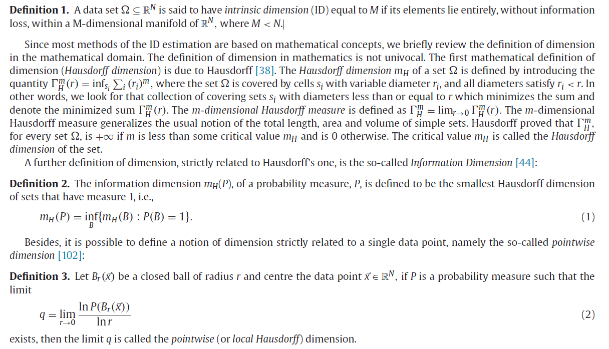
- how to define intrinsic dimension (怎样确定数据在潜藏维度长什么样呢?怎样就规定数据就是在那个维度呢?......)
- and how to estimate it.
The ID estimation methods depend on the scale of data and still suffer from curse of dimensionality (robustness).It is considered to provide a lower bound on the cardinalityinorderto guarantee an accurate ID estimation, however, it is available only for fractal-based methods and Little-Jung-Maggioni's algorithm.
Firstly,
The defination of intrinsic deminsion:
 dimension defination.png-217kB
Secondly,
-
the categories of ID estimation:
-
Global methods use the whole data set making implicitly the assumption that data lie on a unique manifold of a fixed dimen-sionality.
- Global methods can be grouped in five families: projection, multidimensional scaling, fractal-based, multiscale, andother methods, where all the methods that cannot be assigned to the first four kinds of method are collected.
-
Local methods are algorithms that provide an ID estimation using the information contained in sample neighborhoods.
- In this case, data do not lie on a unique manifold of constant dimensionality but on multiple manifolds of different dimensionalities. Since a unique ID estimate for the whole data is clearly not meaningful, it prefers to provide an ID estimate for each small subset of data, assuming that it lies on a manifold of constant dimensionality. Properly, local methods estimate the topological dimension of data manifold. ......The topological dimension is often referred to as the local dimension. For this reason methods that estimate the topological dimension are called local. Local ID estimation methods are Fukunaga-Olsen's, local MDS, local Multiscale, nearest-neighbor algorithms.
-
Pointwise methods, in this category there are the algorithms that can produce both a global ID estimate of the whole data set and local pointwise ID estimate of each pattern of the data set.
- Unlike local methods, where the term local refers to the topological dimension, in pointwise methods local means that the dimension is estimated for the neighborhood of each data sample, thus providing an estimate of pointwise dimension (see the first part). The global ID estimate is given by the mean of pointwise dimension of all patterns of data set.
-
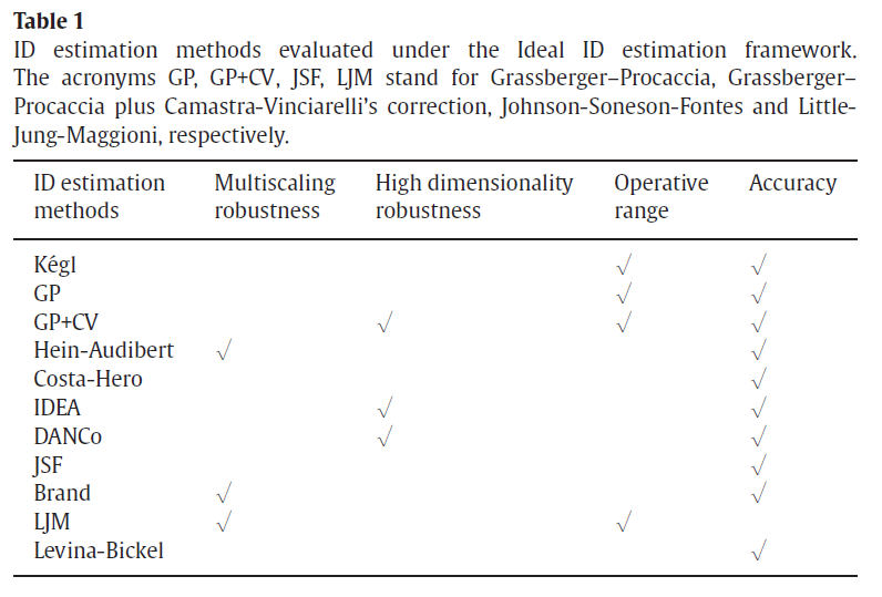
- Meanwhile, the ideal ID estimator is considered to be of the following characters:
- be computational feasible;
- be robust to the multiscaling;
- be robust to the high dimensionality;
- have a work envelope (or operative range);
- be accurate, i.e., give an ID estimate close to the underlying manifold dimensionality (accuracy).
-
ID method evaluaton:
<center>
 ID Method Evaluation.png-75.3kB
</center>
Thirdly,
The more specific description of Fractal-based methods (GP+CV):
-
Fractal-based methods are global methods that were originally proposed in physics to estimate the attractor dimension of nonlinear systems. Since fractals are generally characterized by a non-integer dimensionality (e.g., Koch's curve dimension is $\frac{ln 4}{ln 8}$), these methods are called fractal.
-
Kégl's algorithm
Since Hausdorff dimension is very hard to estimate, fractal methods usually replace it with an upper bound, the Box-Counting Dimension. Let $\Omega = \begin{Bmatrix}\overrightarrow{x_1}, ..., \overrightarrow{x_l}\end{Bmatrix} \subseteq \mathbb{R}^N$ be a data set, we denote by ν(r) the number of the boxes (i.e., hypercubes) of size r required to cover $\Omega$. It can be proved that $ v(r)\propto\frac{1}{r}^M$, where $M$ is the dimension of the set. This motivates the following definition. The Box-Counting Dimension (or Kolmogorov capacity) $M_B$ of the set is defined by
$$M_B = \lim_{r\to 0} \frac{ln(v(r))}{ln(\frac{1}{r})}$$
where the limit is assumed to exist.
Kégl's algorithm is a fast algorithm for estimating the Box-Counting Dimension, however, it does not take into account multiscaling and the high dimensionality robustness. Kégl's algorithm is based on the observation that $ν(r)$ is equivalent to the cardinality of the maximum independent vertex set $MI(G_r)$ of the graph $G_r(V, E)$ with vertex set $V=\Omega$ and edge set $E=\begin{Bmatrix}(\overrightarrow{x_i}, \overrightarrow{x_j}) | d(\overrightarrow{x_i}, \overrightarrow{x_j})<r\end{Bmatrix}$. Kégl proposed to estimate $MI(G)$ using the following greedy approximation. Given a data set $\Omega$, we start with an empty set C. In an iteration over $\Omega$, we add to $C$ data points that are at distance of at least $r$ from all elements of $C$. The cardinality of $C$, after every point in $\Omega$ has been visited, is the estimate of $ν(r)$. The Box-Counting Dimension estimate is given by:
$$M_B = -\frac{ln v(r_2) - ln v(r_1)}{ln r_2 - ln r_1}$$
where $r2$ and $r1$ are values that can be set up heuristically. -
Grassberger–Procaccia algorithm (GP)
A good alternative to the Box-Counting Dimension, among many proposed is the Correlation Dimension, defined as follows. If the correlation integral $C(r)$ is given by:
$$C(r) = \lim_{l\to \infty}\frac{2}{l(l-1)} \sum_{i=1}^{l} \sum_{j=i+1}^{l} I( \begin{Vmatrix}\overrightarrow{x_j}- \overrightarrow{x_i} \end{Vmatrix}\leq r)$$
where $I$ is an indicator function (i.e., it is 1 if condition holds, 0 otherwise), then the Correlation Dimension Mc of $\Omega$ is:
$$M_B = \lim_{r\to 0} \frac{ln(C(r))}{ln(r)}$$
It can be proved that the Correlation Dimension is a lower bound of the Box-Counting Dimension. The most popular method to estimate Correlation Dimension is the Grassberger–Procaccia algorithm. This method consists in plotting $ln (C_m(r))$ versus $ln (r)$. The Correlation Dimension is the slope of the linear part of the curve. -
Takens' method
Takens proposed a method, based on the Maximum Likelihood principle, that estimates the expectation value of Correlation Dimension. Let $Q = \begin{Bmatrix}q_k|q_k<r\end{Bmatrix}$ be the set formed by the Euclidean distances (denoted by $q_k$), between data points of $\Omega$, lower than the so-called cut-off radius $r$. Using the Maximum Likelihood principle Takens proved that the expectation value of the Correlation Dimension $\left\langle M_c \right\rangle$ is:
$$ \left\langle M_c \right\rangle = -(\frac{1}{|Q|} \sum_{k=1}^{|Q|}q_k )^{-1} $$
where $|Q|$ denotes the cardinality of $Q$. Takens' method presents some drawbacks. Firstly, the cut-off radius can be set only by using some heuristics. Besides, the method is optimal only if the correlation integral C(r) has the form $C(r)= \alpha r^D[1+ \beta r^2 + o(r^2)]$ where $\alpha, \beta \in \mathbb{R}^+$ -
Work envelope of fractal-based methods
Differently from the other ID methods described before, fractal-based methods satisfy, in addition to the third one, the fourth Ideal ID requirement, i.e., they have a work envelope. They provide a lower bound that the cardinality of data set must fulfill in order to get an accurate ID estimate. Eckmann and Ruelle proved that to get an accurate estimate of the dimension M,the data set cardinality has to satisfy the following inequality:
$$M<2\log_{10}l$$
which shows that the number of data points required to estimate accurately the dimension of a M-dimensional set is at least $10^{\frac{M}{2}}$. Even for sets of moderate dimension this leads to huge values of $l$.To improve the reliability of the ID estimate when the cardinality $l$ does not fulfill the inequality, the method of surrogate data was proposed. The method of surrogate data is based on bootstrap. Given a dataset $\Omega$, the method consists in creating a new synthetic data set $\Omega'$, with larger cardinality, that has the same mean, variance and Fourier Spectrum of $\Omega$. Although the cardinality of $\Omega'$ can be chosen arbitrarily, the method of surrogate data becomes infeasible when the dimensionality of the data set is high. For instance, a 50-dimensional data set to be estimated must have at least $10^{25}$ data points, on the basis of the inequality.
-
Camastra–Vinciarelli's algorithm (CV)
For the reasons described above, Fractal-based algorithms do not satisfy the third Ideal ID requirement, i.e., they do not provide reliable ID estimate when the cardinality of the data set is high. In order to cope with this problem, Camastra and Vinciarelli proposed an algorithm to power Grassberger and Procaccia method (GP method) w.r.t. high dimensionality, evaluating empirically how much the GP method underestimates the dimensionality of a data set when the data set cardinality is unadequate to estimate ID properly. Let $\Omega = \begin{Bmatrix}\overrightarrow{x_1}, ..., \overrightarrow{x_l}\end{Bmatrix} \subseteq \mathbb{R}^N$ be a data set, Camastra–Vinciarell's algorithm has the following steps:
-
Create a set $\Omega'$, whose ID M is known, with the same cardinality $l$ of $\Omega$. For instance, $\Omega'$ could be composed of data points randomly generated in a M-dimensional hypercube.
-
Measure the Correlation Dimension Mc of $\Omega'$ by the GP method.
-
Repeat the two previous steps for T different values of M, obtaining the set $C = \begin{Bmatrix}(M_i, M^{i}_{c}) : i = 1, 2,...,T\end{Bmatrix}$.
-
Perform a best fitting of data in C by a nonlinear method. A plot (reference curve) $P$ of $M_c$ versus $M$ is generated. The reference curve allows inferring the value of $M_c$ when $M$ is known.
-
The Correlation Dimension $M_c$ of $\Omega$ is computed by the GP method and, by using $P$, the ID of $\Omega$ can be estimated.
The algorithm assumes that the curve $P$ depends on and its dependence on sets are negligible. It is worth mentioning that OganovandValle used Camastra–Vinciarelli's algorithm to estimate ID of high dimensional Crystal Fingerprint spaces.
-


网友评论