差异表达基因检测 | DESeq2

写在前面

前面用EBSeq做完2 cases vs.2 controls的分析，得到的DEG屈指可数（~200个），觉得怪怪的。所以重新查了下资料，说是EBSeq比较依赖于样本量，相对保守。只有2个重复的样本来说，用DESeq2得挺多。

DESeq2是DESeq的进阶版

DESeq method detects and corrects dispersion estimates that are too low through modeling of the dependence of the dispersion on the average expression strength over all samples.
DESeq2, a method for differential analysis of count data, using shrinkage estimation for dispersions and fold changes to improve stability and interpretability of estimates. This enables a more quantitative analysis focused on the strength rather than the mere presence of differential expression.
The package DESeq2 provides methods to test for differential expression by use of negative binomial generalized linear models; the estimates of dispersion and logarithmic fold changes incorporate data-driven prior distributions.

负二向分布有两个参数，均值(mean)和离散值（dispersion). 离散值描述方差偏离均值的程度。泊松分布可以认为是负二向分布的离散值为1，也就是均值等于方差（mean=variance）的情况。
manual: https://bioconductor.org/packages/release/bioc/vignettes/DESeq2/inst/doc/DESeq2.html

实战

input文件是un-normalized counts。DESeq2的统计模型用un-normalized counts是最powerful的，软件内部会根据library size differences进行校正。

如何获得un-normalized counts?
参考http://master.bioconductor.org/packages/release/workflows/vignettes/rnaseqGene/inst/doc/rnaseqGene.html。

不同的方法(summarizeOverlaps, featureCOunts, tximport, htseq-count)得到的count数据，DESeq2在导入数据时使用的函数不同，具体见文档啦。
这里使用htseq-count计算counts，每个样本得到一个单独的结果文件，可以使用其对应DESeq2的函数是DESeqDataSetFromHTSeq导入数据。更快捷的方法是在linux将文件合并后输入。

安装

source("https://bioconductor.org/biocLite.R")
biocLite("DESeq")
biocLite("DESeq2")
biocLite("limma")
biocLite("pasilla")
biocLite("vsn")
biocLite("IHW")

Example

#input files
  #cts: a count matrix 
  #coldata:a table of sample information 
library("pasilla")
pasCts <- system.file("extdata",
                      "pasilla_gene_counts.tsv",
                      package="pasilla", mustWork=TRUE)
pasAnno <- system.file("extdata",
                       "pasilla_sample_annotation.csv",
                       package="pasilla", mustWork=TRUE)
cts <- as.matrix(read.csv(pasCts,sep="\t",row.names="gene_id"))
coldata <- read.csv(pasAnno, row.names=1)
coldata <- coldata[,c("condition","type")]

  #cts和coldata的samples顺序必须一致，DESeq2不会自动判断
rownames(coldata) <- sub("fb", "", rownames(coldata))  #修改coldata的rownames
all(rownames(coldata) %in% colnames(cts))
cts <- cts[, rownames(coldata)]  #将cts的列，按照coldata顺序排列
all(rownames(coldata) == colnames(cts))  #check两者顺序是否一致

coldata
#condition        type
#treated1     treated single-read
#treated2     treated  paired-end
#treated3     treated  paired-end
#untreated1 untreated single-read
#untreated2 untreated single-read
#untreated3 untreated  paired-end
#untreated4 untreated  paired-end
head(cts,2)
#treated1 treated2 treated3 untreated1 untreated2 untreated3 untreated4
#FBgn0000003        0        0        1          0          0        0          0
#FBgn0000008      140       88       70         92        161        76         70

#construct a DESeqDataSet
require("DESeq2")
dds <- DESeqDataSetFromMatrix(countData = cts,
                              colData = coldata,
                              design = ~ condition)

#pre-filtering:去除read counts很少的基因,这里要求每个基因在所有个体中的reads数之和>=10。结果部分会使用更严格的过滤条件
keep <- rowSums(counts(dds)) >= 10
dds <- dds[keep,]
  #指定factor level：告诉软件谁是control，有以下两种方法
dds$condition <- factor(dds$condition, levels = c("untreated","treated"))
dds$condition <- relevel(dds$condition, ref = "untreated")

#Differential expression analysis
dds <- DESeq(dds)
res <- results(dds)  #此时，默认过滤(adjp<=0.1)
#resNoFilt <- results(dds, independentFiltering=FALSE) #不过滤

  #提取想要的差异分析结果，我们这里是treated组对untreated组进行比较
res <- results(dds, contrast=c("condition","treated","untreated"))

  #Log fold change shrinkage for visualization and ranking
resultsNames(dds)
#use the apeglm method for effect size shrinkage (Zhu, Ibrahim, and Love 2018), which improves on the previous estimator.
resLFC <- lfcShrink(dds, coef="condition_treated_vs_untreated", type="apeglm")

  #按p value 升序排序并输出，也可以按padj排序
resOrdered <- res[order(res$pvalue),]
  #How many adjusted p-values were less than 0.1?
sum(res$padj < 0.1, na.rm=TRUE)
  #results会自动进行过滤，仅保留adjusted p value <0.1 的基因,如果需要修改，更改alpha参数即可
res05 <- results(dds, alpha=0.05)
summary(res05)

#可视化
x=as.data.frame(res)
plotMA(x, ylim=c(-2,2))

#结果输出
write.csv(as.data.frame(res),file="condition_treated_results.csv") #所有结果
mcols(res)$description #res各项结果说明
  #提取padj<0.1的数据
resSig <- subset(resOrdered, padj < 0.1)
write.csv(as.data.frame(resSig),file="condition_treated_results.csv") #所有结果

分析前的质量评估
主要看下样本之间重复性如何，标准化前后的效果等。

library("pheatmap")
select <- order(rowMeans(counts(dds,normalized=TRUE)),
                decreasing=TRUE)[1:20]   #降序排列后，提取1-20行
df <- as.data.frame(colData(dds)[,c("condition","type")])
ntd <- normTransform(dds) #数据标准化(有多种方法)：the transformed data, across samples, against the mean, using the shifted logarithm transformation
vsd <- vst(dds, blind=FALSE) #数据标准化: the regularized log transformation 
rld <- rlog(dds, blind=FALSE) #数据标准化: the variance stabilizing transformation

#标准化前后的比较
par(mfrow=c(2,2))
boxplot(assay(dds))
boxplot(assay(rld))
hist(assay(dds))
hist(assay(rld))

library("vsn")
pheatmap(assay(ntd)[select,], cluster_rows=FALSE, show_rownames=FALSE,
         cluster_cols=FALSE, annotation_col=df) #调节参数

#Heatmap of the sample-to-sample distances:an overview over similarities and dissimilarities between samples.
sampleDists <- dist(t(assay(vsd)))
library("RColorBrewer")
sampleDistMatrix <- as.matrix(sampleDists)
rownames(sampleDistMatrix) <- paste(vsd$condition, vsd$type, sep="-")
colnames(sampleDistMatrix) <- NULL
colors <- colorRampPalette( rev(brewer.pal(9, "Blues")) )(255)
pheatmap(sampleDistMatrix,
         clustering_distance_rows=sampleDists,
         clustering_distance_cols=sampleDists,
         col=colors)

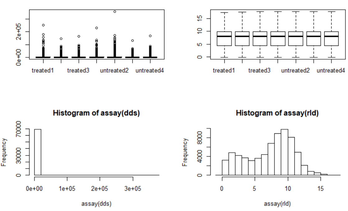标准化前后（左前右后）

实际数据

01 输入文件：combined.count
genes X read_counts的表格，如下

gene    EGFP1   EGFP2   KD1 KD2
ENSMUSG00000000001  295 233 281 243
···

02 读入数据

require("DESeq")
require("DESeq2")
require("limma")
require("pasilla")
require("vsn")  

data=read.table("combined.count",header=T,row.names=1)
head(data,3)

condition = factor(rep(c("EGFP","KD"),each=2))
coldata <- data.frame(condition)
rownames(coldata) = c("EGFP1","EGFP2","KD1","KD2")
coldata
 #condition
 #EGFP1      EGFP
 #EGFP2      EGFP
 #KD1          KD
 #KD2          KD
all(rownames(coldata)==colnames(data))   #检查coldata和data的样本名称及顺序是否一致

require("DESeq2")
ds<-DESeqDataSetFromMatrix(countData=data,colData=coldata,design = ~ condition)

03 数据过滤及评估

#pre-filtering
keep <- rowSums(counts(ds))>=10
ds <- ds[keep,]
nrow(ds) #剩余多少gene
ds$condition <- relevel(ds$condition,ref="EGFP") #指定对照组

#预评估
#01 数据标准化前后的比较: the variance stabilizing transformation(这里使用rlog进行标准化)
rld <- rlog(ds, blind=FALSE) 
par(mfrow=c(2,2))
boxplot(assay(ds))
boxplot(assay(rld))
hist(assay(ds))
hist(assay(rld))

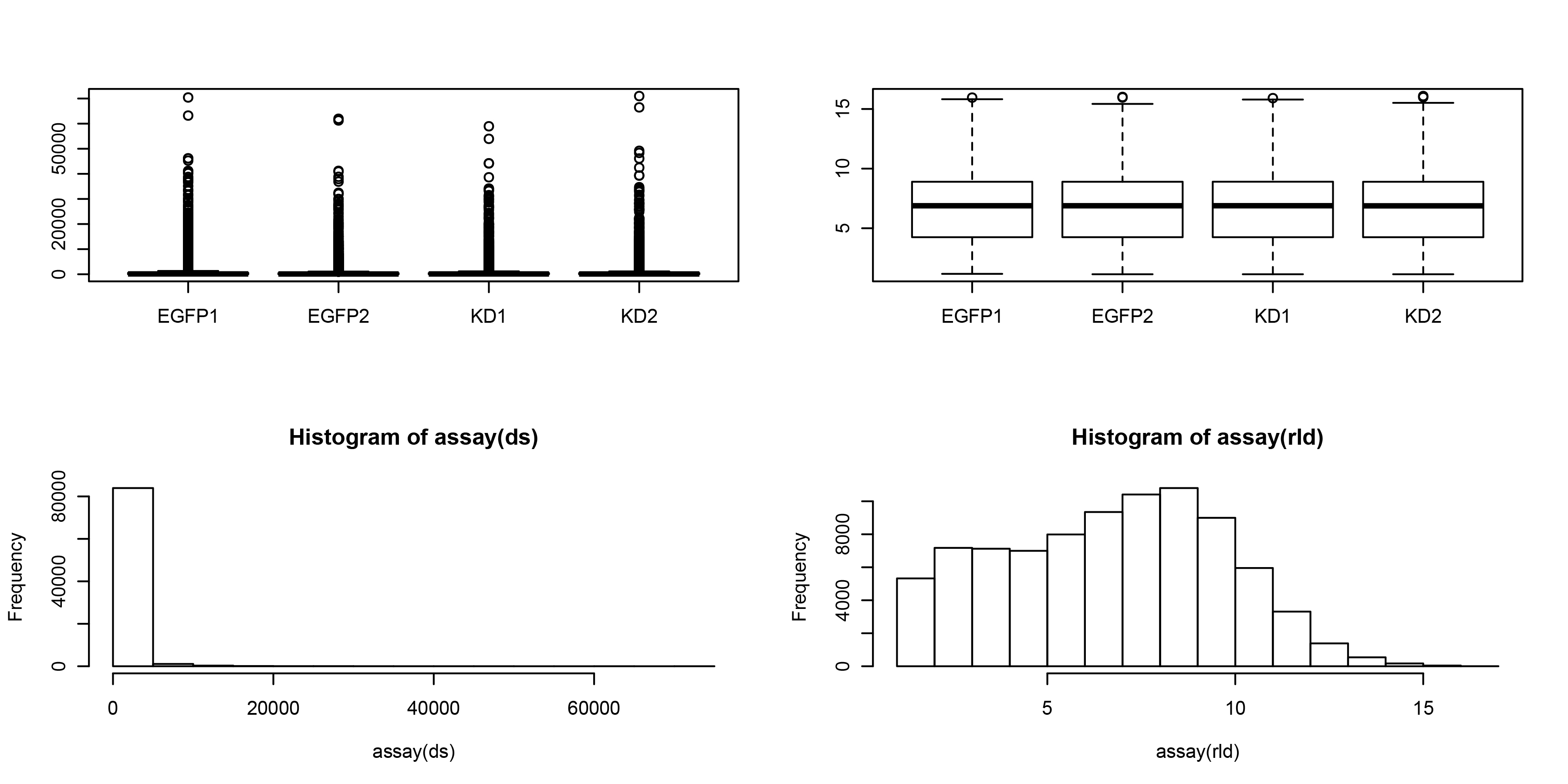标准化前（左）后（右）比较

#02 对标准化后的数据进行聚类-heatmap
df <- as.data.frame(colData(ds)[,c("condition")])
rownames(df)=c("EGFP1","EGFP2","KD1","KD2")
colnames(df)=c("condition")
require(pheatmap)
p1=pheatmap(assay(rld), cluster_rows=FALSE, show_rownames=FALSE,
         cluster_cols=TRUE, annotation_col=df) #显示所有基因的数据，并按样本聚类
require(Cairo)
Cairo( width = 640, height = 480,type="png",file="heatmap_all.png",
pointsize = 12, res=100)
p1
dev.off()
#提取部分基因的信息进行聚类
select <- order(rowMeans(counts(ds,normalized=TRUE)),
                decreasing=TRUE)[1:20]   #降序排列后，提取1-20行
pheatmap(assay(rld)[select,], cluster_rows=FALSE, show_rownames=FALSE,
         cluster_cols=TRUE, annotation_col=df) #按提取的20行进行聚类

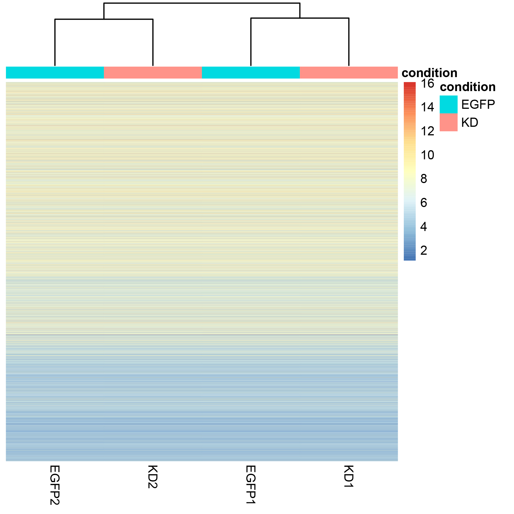heatmap

#03 计算样本间的距离:sampe vs. sample
sampleDists <- dist(t(assay(rld)))
require("RColorBrewer")
sampleDistMatrix <- as.matrix(sampleDists)
rownames(sampleDistMatrix) <- colnames(rld)
colnames(sampleDistMatrix) <- colnames(rld)
colors <- colorRampPalette( rev(brewer.pal(9, "Blues")) )(255)
p2=pheatmap(sampleDistMatrix,
         clustering_distance_rows=sampleDists,
         clustering_distance_cols=sampleDists,
         col=colors)
Cairo( width = 480, height = 480,type="png",file="distance.png",
pointsize = 12, res=100)   
p2
dev.off()

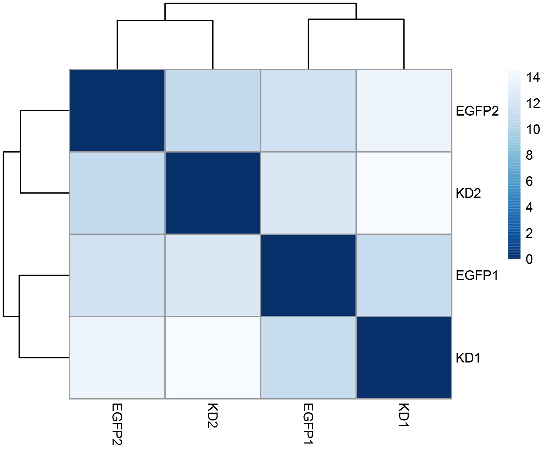distance

04 差异表达基因检测

#differential expression analysis
ds <- DESeq(ds)
res <- results(ds)
res <- results(ds,contrast = c("condition","KD","EGFP")) 

#看总体情况：多少上调，多少下调
summary(res)
#out of 21396 with nonzero total read count
#adjusted p-value < 0.1
#LFC > 0 (up)       : 87, 0.41%
#LFC < 0 (down)     : 270, 1.3%
#outliers [1]       : 0, 0%
#low counts [2]     : 14933, 70%
#(mean count < 360)

#统计p adj<0.1的基因数目
sum(res$padj<0.1,na.rm=TRUE) 

#reorder by p-adj
resOrdered <- res[order(res$padj),]

#可视化
#没有经过 statistical moderation平缓log2 fold changes的情况
plotMA(res, ylim = c(-5,5))
topGene <- rownames(res)[which.min(res$padj)]
with(res[topGene, ], {
  points(baseMean, log2FoldChange, col="dodgerblue", cex=2, lwd=2)
  text(baseMean, log2FoldChange, topGene, pos=2, col="dodgerblue")
})
#经过lfcShrink 收缩log2 fold change
resLFC <- lfcShrink(ds,coef="condition_KD_vs_EGFP",type="apeglm")
plotMA(resLFC, ylim = c(-5,5))
topGene <- rownames(res)[which.min(res$padj)]
with(res[topGene, ], {
  points(baseMean, log2FoldChange, col="dodgerblue", cex=2, lwd=2)
  text(baseMean, log2FoldChange, topGene, pos=2, col="dodgerblue")
})

#结果输出
mcols(res)$description #res各项结果说明
#输出所有结果
write.csv(as.data.frame(res),file="DEG_KDvsEGFP_all.csv") 
#提取差异表达的基因padj<0.05的数据
resSig <- subset(res, padj < 0.05)
write.csv(as.data.frame(resSig),file="DEG_005.csv") 

根据输出的结果，按照p-adj进行筛选。

这里p-adj校正时使用的是multiple test correction，根据文献，推荐使用Independent Hypothesis Weighting (IHW)。参考 https://www.michaelchimenti.com/2017/02/beyond-benjamini-hochberg-multiple-test-correction-with-independent-hypothesis-weighting-ihw/
Independent Hypothesis Weighting (IHW) 校正的具体操作如下：

library("IHW")
resIHW <- results(ds, filterFun=ihw)
summary(resIHW)
sum(resIHW$padj < 0.1, na.rm=TRUE)
sum(resIHW$padj < 0.05, na.rm=TRUE)
metadata(resIHW)$ihwResult
write.csv(as.data.frame(resIHW),file="DEG_KDvsEGFP_all_resIHW.csv") 
mcols(resIHW)$description #结果列说明

Note : 为啥这么多p-adj是NA？
查看所有基因的输出结果，你可能会遇到这种情况：许多基因的p-value很显著，p-adj是NA，而baseMean并不低。这是因为results函数会对结果进行independent filtering，而且是用normalized counts的平均值来进行筛选，这个值是根据显著性水平alpha(默认值是0.1，也就是p-adj）来确定的。
其实在summary(res)查看结果时，就可以看到具体的值，比如下面的结果显示有70%的属于low counts,也就是mean count<360，因此其p-adj就被设置为NA。可以用independentFiltering关掉independent filtering.可以看到结果会有一些差异。

resNoFilt <- results(dds, independentFiltering=FALSE)
write.csv(as.data.frame(resNoFilt),file="DEG_KDvsEGFP_all_resNoFilt.csv")  #输出看看，只是给出了p-adj，然而都是>0.1，所以，前面的操作没毛病。
addmargins(table(filtering=(res$padj < .1),
                 noFiltering=(resNoFilt$padj < .1)))
#          noFiltering
#filtering FALSE TRUE  Sum
#    FALSE  6106    0 6106
#    TRUE    214  143  357
#    Sum    6320  143 6463